Analyzing multiple TMT plexes with FragPipe
FragPipe includes TMT-Integrator, which filters and combines isobaric quantification information (from psm.tsv reports generated by Philosopher) into reports at many levels: gene, protein, peptide, and modification site. It can be used on a single multiplexed sample (e.g. one TMT 10-plex) or to integrate quantification information across many multiplexed samples, with the option to use a pooled reference channel (or a virtual one if a pooled reference channel has not been included in the experiment). This tutorial analyzes two TMT10-labeled plexes, each with one TMT channel that contains a pooled reference sample.
These data are part of a kidney clear cell carcinoma dataset from the Clinical Proteomic Tumor Analysis Consortium (CPTAC), where patient samples have been labeled with the TMT 10-plex reagent. These data were acquired on an Orbitrap Fusion Lumos, and the full dataset is publicly available from the CPTAC data portal. It includes both samples that were phosphopeptide-enriched and samples that are unenriched (whole proteome), this tutorial will analyze a subset of each, starting with the phosphopeptides.
Associated publication: Clark, David J., et al. “Integrated proteogenomic characterization of clear cell renal cell carcinoma.” Cell 179.4 (2019): 964-983.
Tutorial contents
- Open FragPipe
- Load the data
- Load the TMT phospho workflow
- Fetch a sequence database
- Inspect the search and quantification settings
- Set output location and run
- Inspect the phospho results
- Analyze the whole proteome samples
Open FragPipe
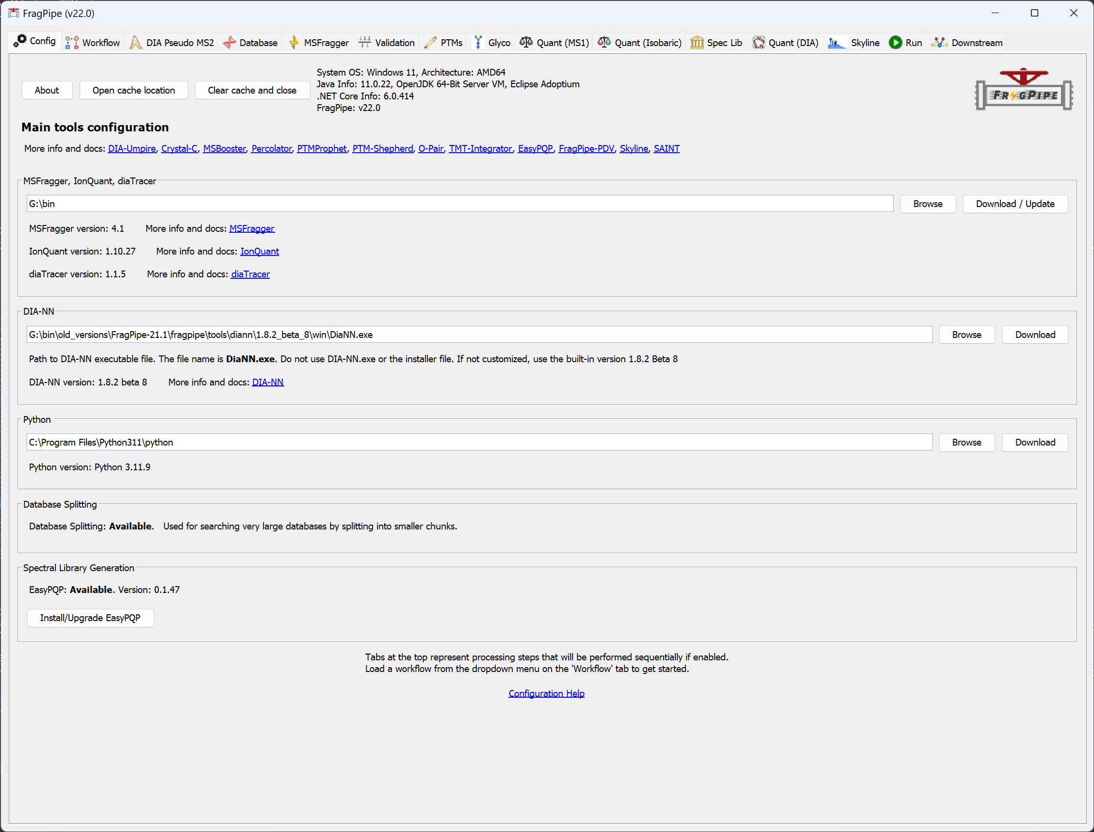
When you launch FragPipe, check that MSFragger, IonQuant, and Philosopher are configured. (If you haven’t downloaded them yet, use their respective ‘Download / Update’ buttons. See this page for more help, Python is not needed for the exercises in this tutorial.)
Load the data
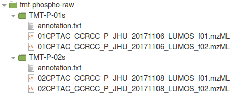
For this tutorial, we will download 01CPTAC_CCRCC_P_JHU_20171106_LUMOS_f01.raw, 01CPTAC_CCRCC_P_JHU_20171106_LUMOS_f02.raw, 02CPTAC_CCRCC_P_JHU_20171108_LUMOS_f01.raw, and 02CPTAC_CCRCC_P_JHU_20171108_LUMOS_f02.raw from CPTAC data portal and convert them to .mzML format (from .raw, conversion tutorial here), and organized into subfolders by plex (two high-pH fractions per plex/folder) with corresponding TMT channel annotation files. The file organization is shown below, where ‘TMT-P-01s’ and ‘TMT-P-02s’ are the two plexes and ‘f01’ and ‘f02’ indicate two fractions of the same 10-plex. Different plexes must be organized into separate, uniquely-named folders as shown in this example.
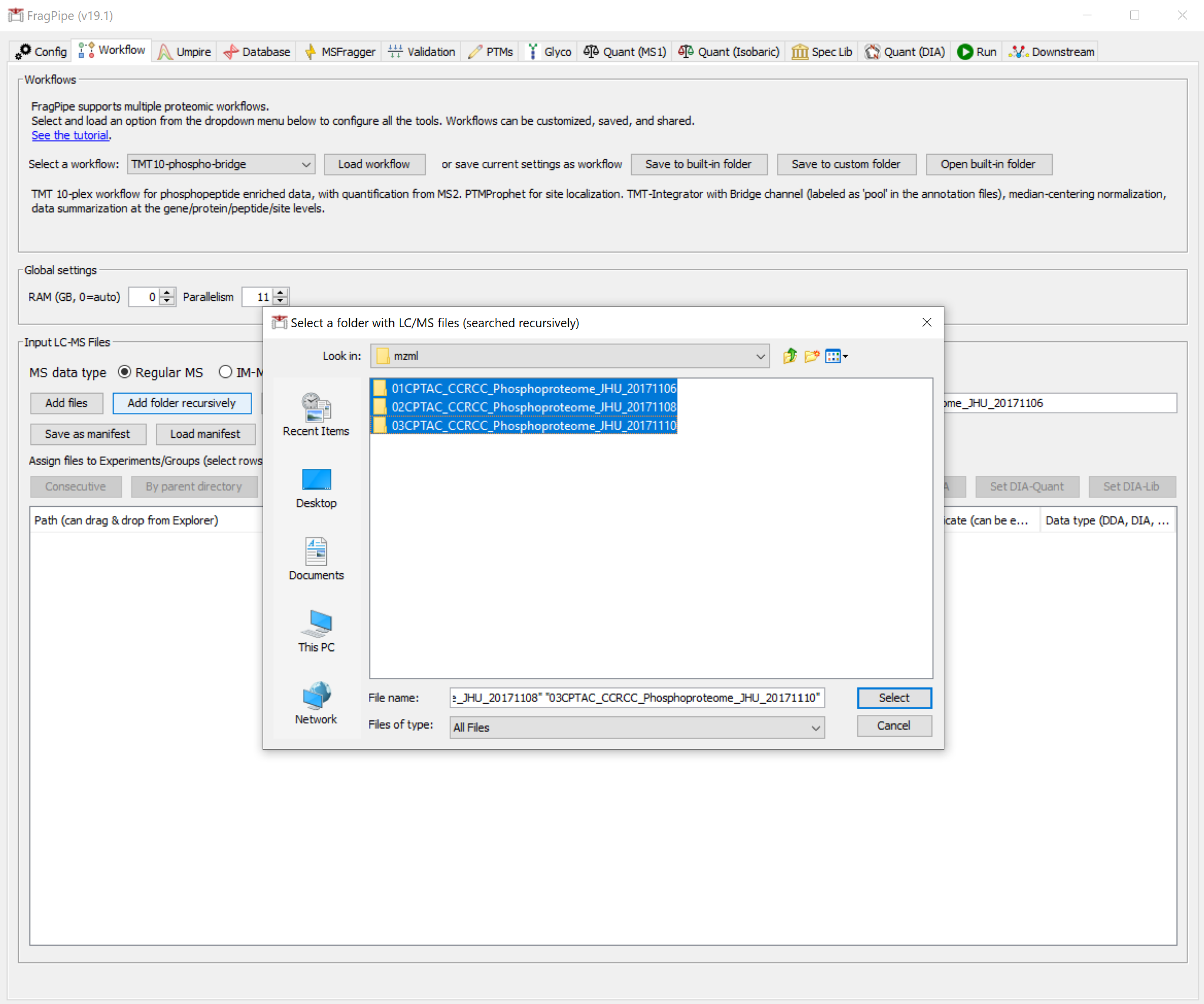
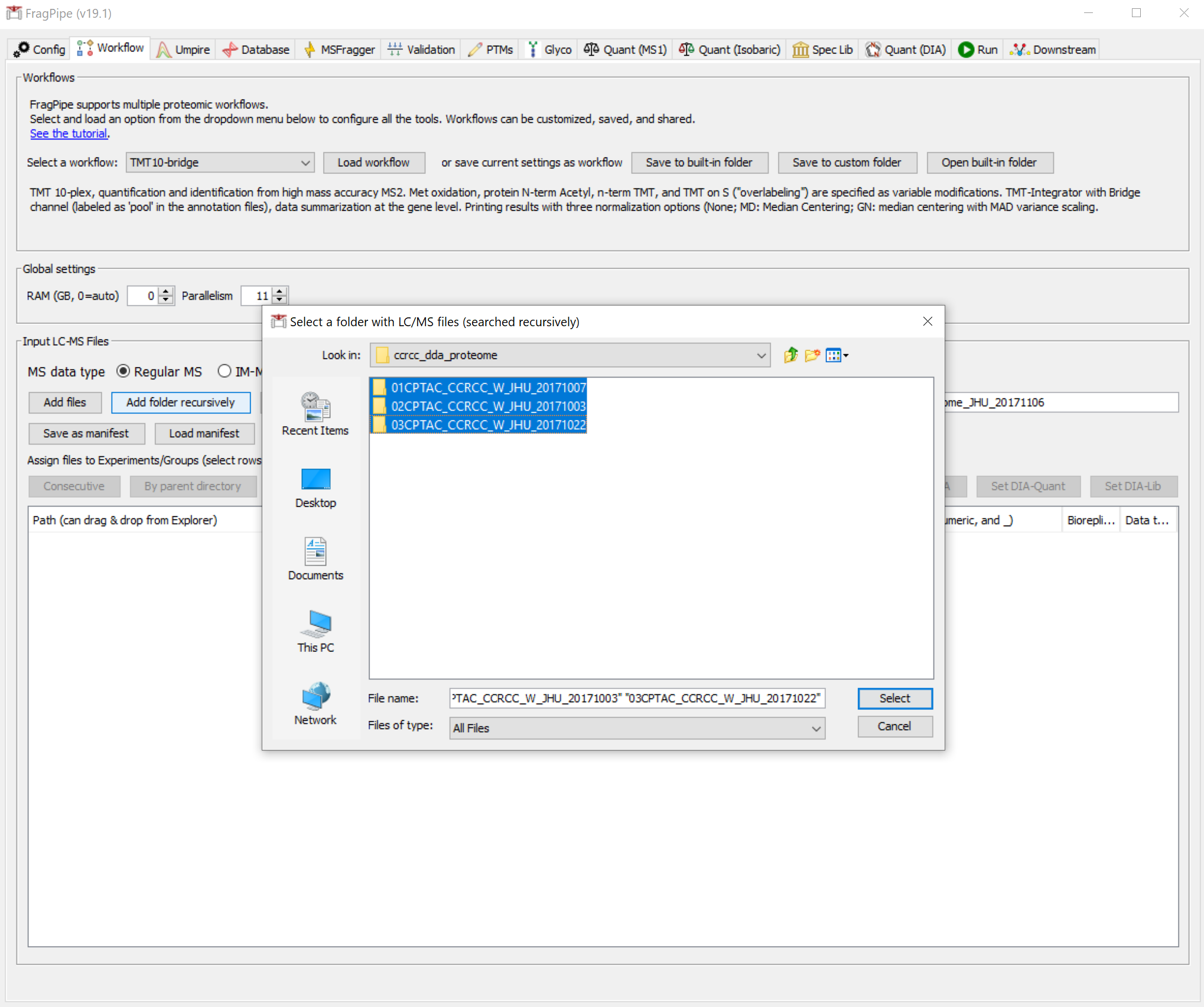
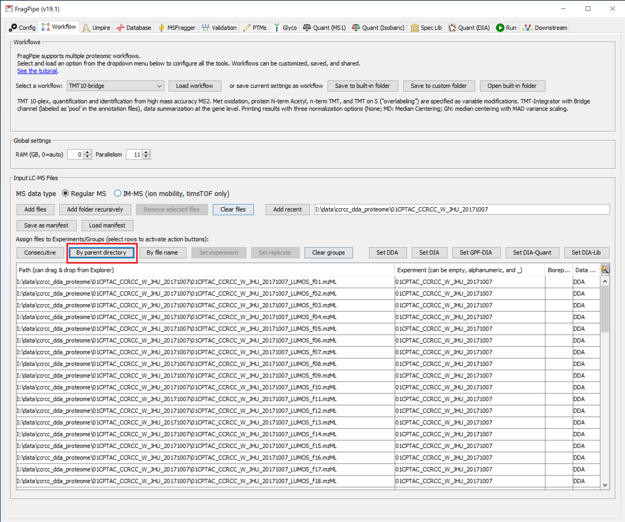
On the ‘Workflow’ tab, use the ‘Add folder recursively’ button to browse and select the ‘tmt-phospho-raw’ folder.
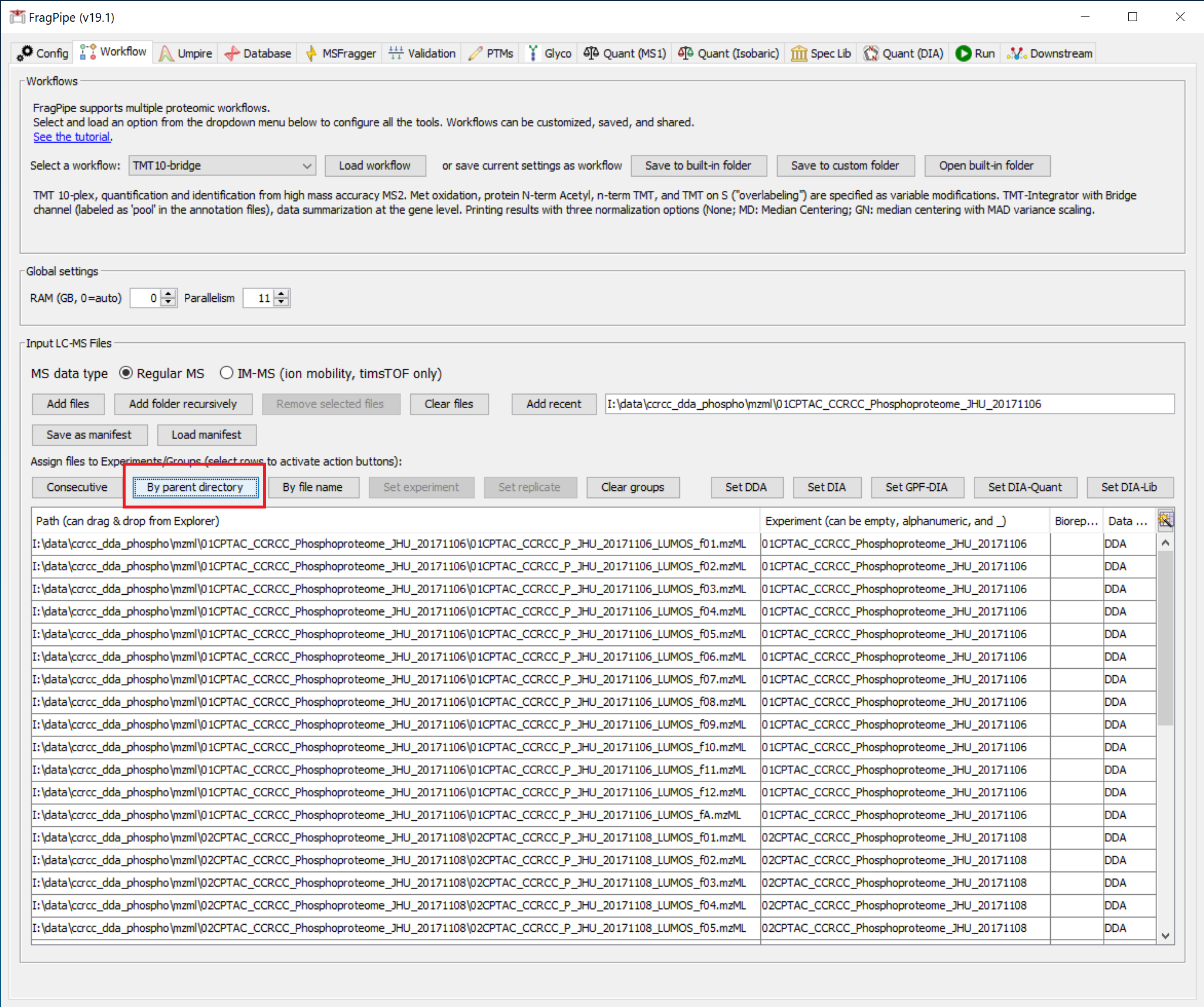
Four .mzML spectral files should be loaded. Then use the ‘By parent directory’ button to assign experiment names to the files by the folder name. The result should look like this:
Load the TMT phospho workflow
On the ‘Workflow’ tab, select the ‘TMT10-phospho-bridge’ workflow from the dropdown menu, press ‘Load’, and confirm.

This sets all the analysis steps for a closed database search with MSFragger (including the appropriate TMT-10 modification settings); validation, filtering, and isobaric quantification with Philosopher; and TMT report generation with TMT-Integrator.
Fetch a sequence database
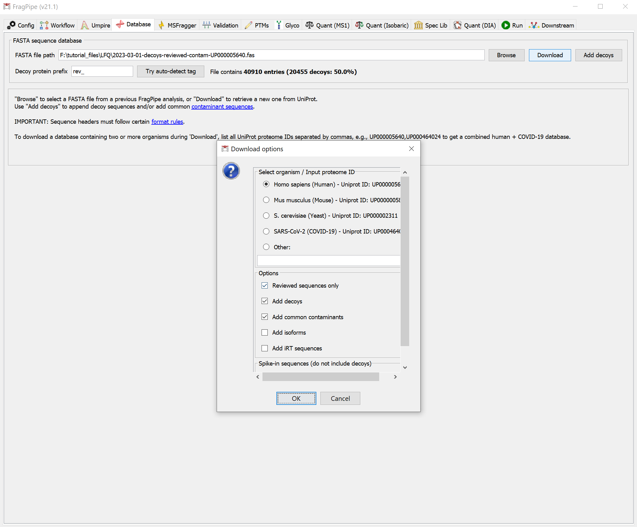
If you haven’t already downloaded a FASTA sequence database with FragPipe, go to the ‘Database’ tab and use the ‘Download’ button to retrieve sequences from UniProt.
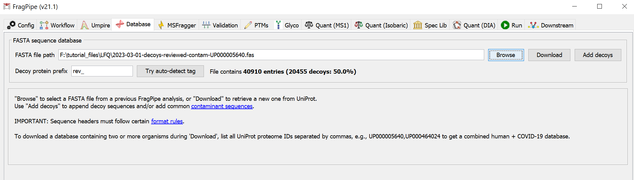
You will need to select a download location first before proceeding to fetch the database with the default options (reviewed human sequences plus common contaminants).
Inspect the search and quantification settings
On the ‘MSFragger’ tab, you can see the parameters that have been set by loading the TMT-10 phospho workflow. Phosphorylation is set as a variable modification, and TMT labeling of the peptide N-terminus and lysine are set as fixed modifications.
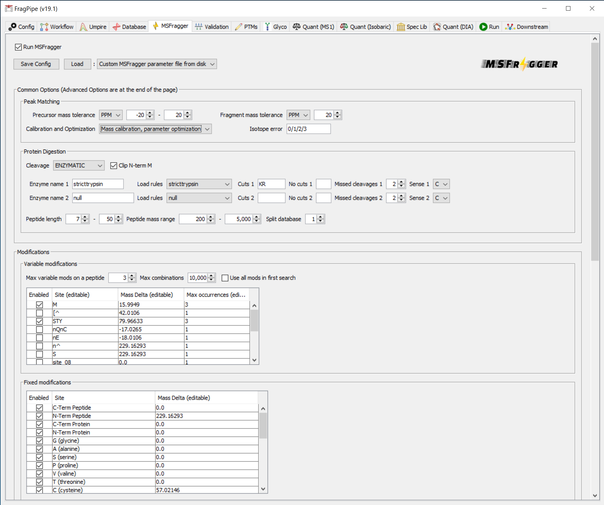
To save time in the search (at the expense of slightly lower sensitivity), you can optionally set ‘Calibration and Optimization’ to ‘None’ in the ‘Peak Matching’ section.
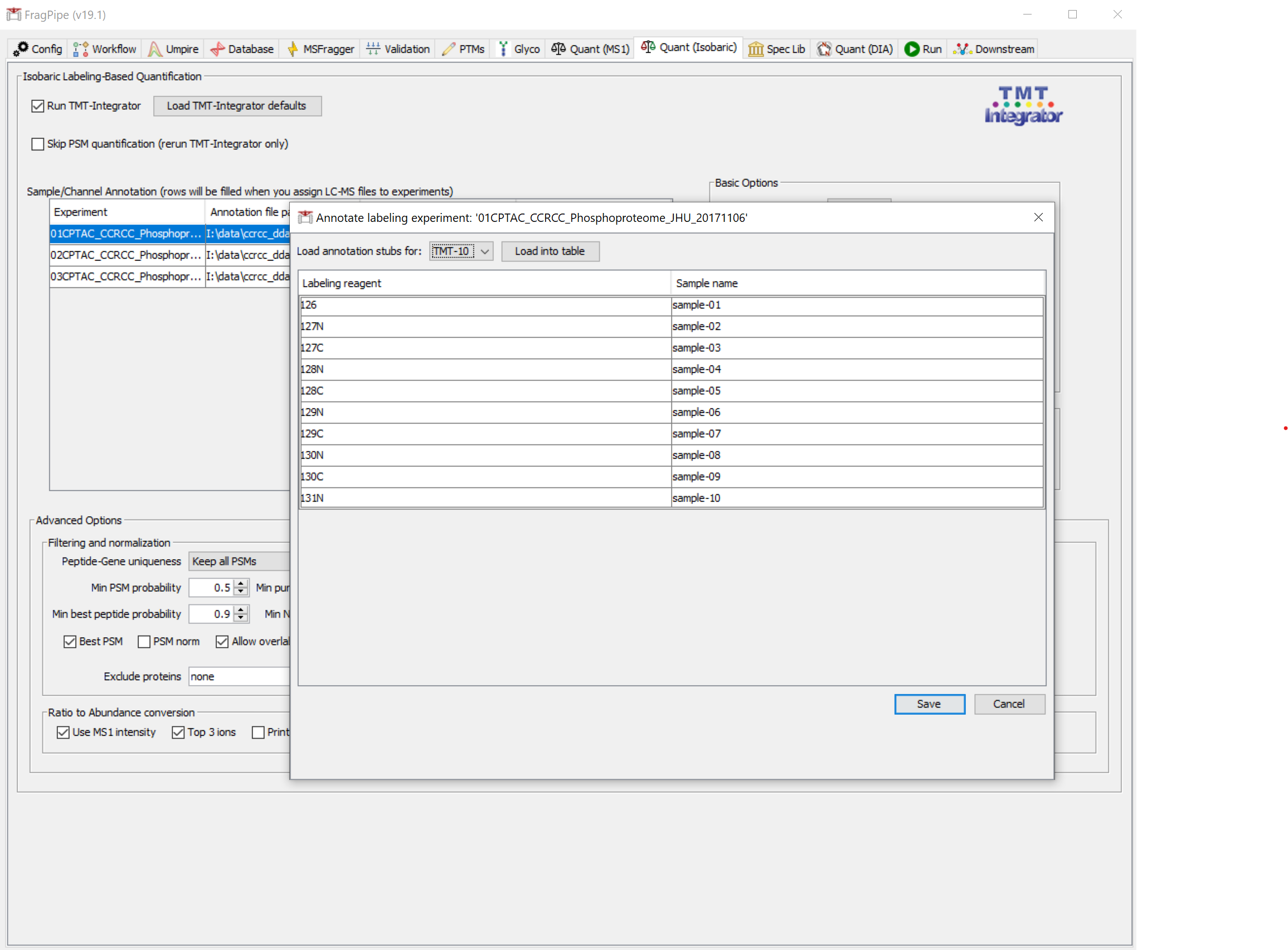
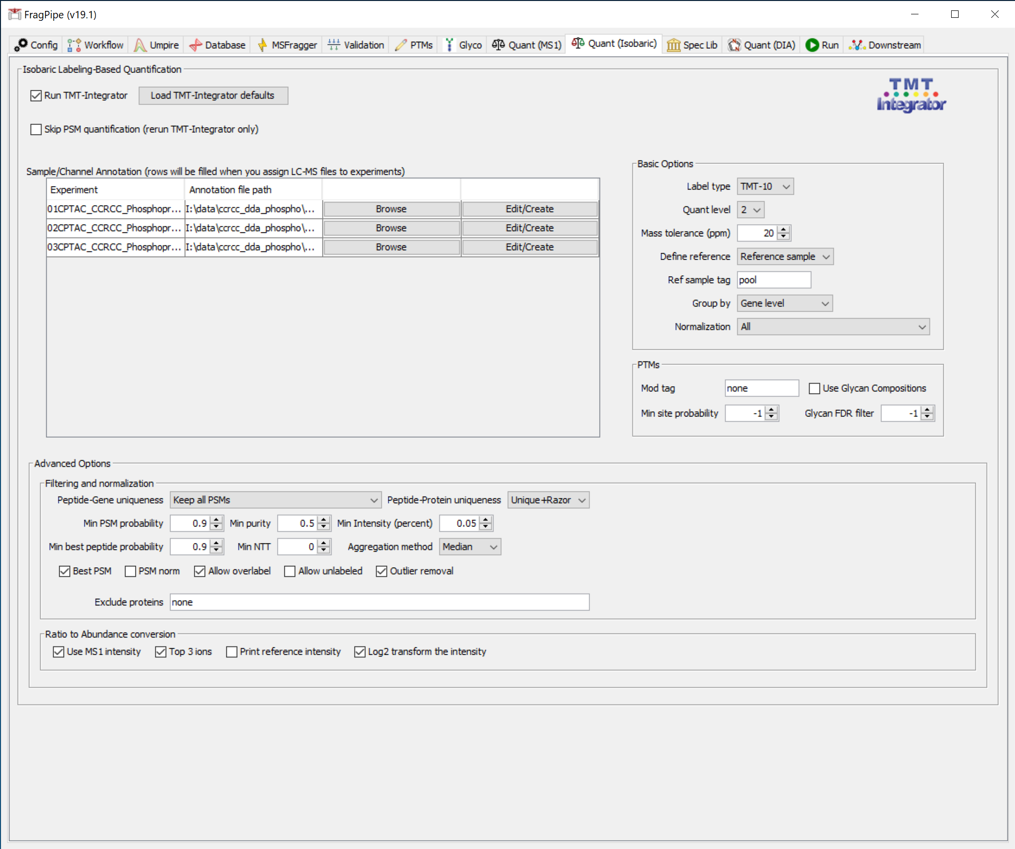
On the ‘Quant (Isobaric)’ tab, you should see that TMT quantification settings for 10-plex labeling have been set, and the TMT channel annotation files have been automatically loaded (they are named ‘annotation.txt’ in this case, but any file ending in ‘annotation.txt’ will be automatically loaded from the same folder as the mzML files). Note that a reference sample is included in this dataset, with the sample tag ‘pool’.
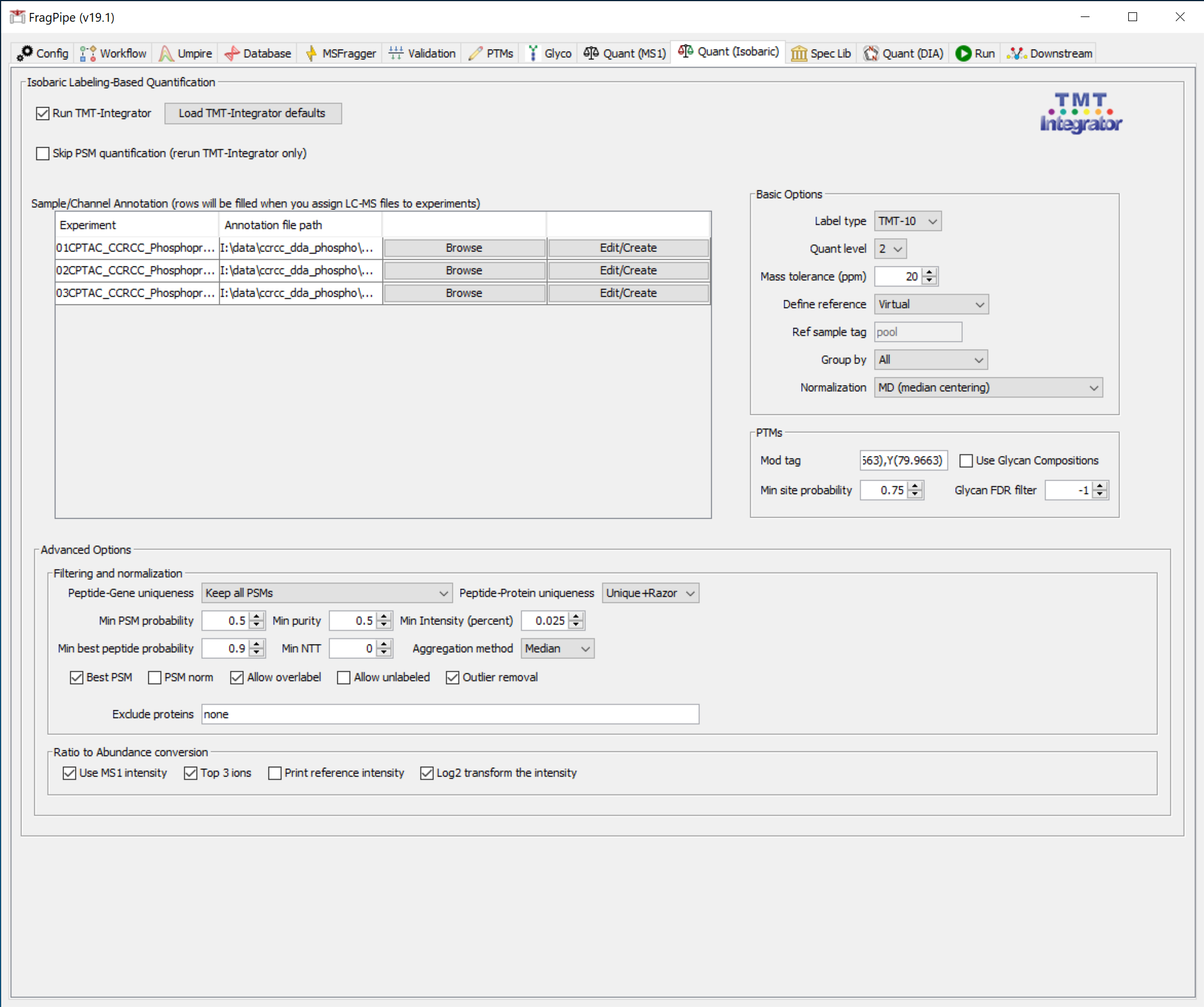
You can inspect the channel annotations by clicking ‘Edit/Create’ for one of the plexes. Note that the pool sample in the ‘TMT-P-02s’ plex is labeled ‘pool02’– each pooled sample is given a unique name, but still needs to contain the tag ‘pool’.
Set output location and run
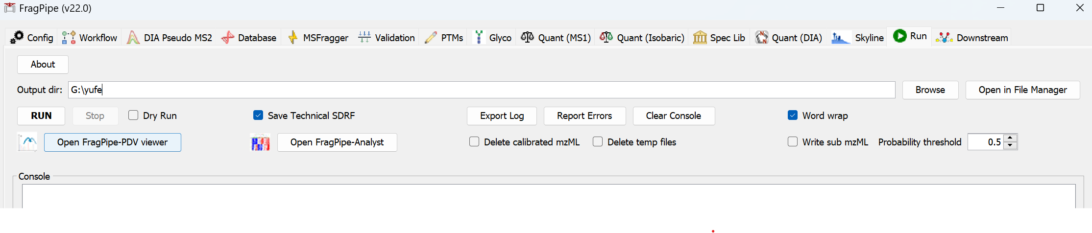
On the ‘Run’ tab, use ‘Browse’ to make a new folder for the output files (e.g. ‘my-tmt-phospho-results’). Then click the ‘RUN’ button to start the analysis.
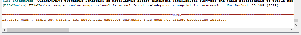
When the run is finished, ‘DONE’ will be printed at the end of the text in the console.
Inspect the phospho results
In the output location (‘my-tmt-phospho-results’ folder), you will find folders containing reports for each plex individually as well as the ‘tmt-report’ folder containing combined quantification reports.
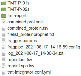
The contents of the ‘tmt-report’ folder are shown below. Reports at the gene, protein, peptide, and phosphosite levels have been generated. A more detailed guide to these output files can be found here.
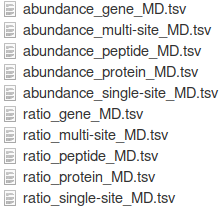
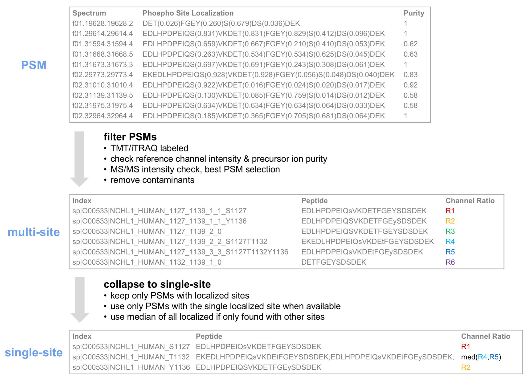
Multi-site and single-site reports will be generated for the specified modification, in this case phosphorylation. In single-site reports, peptides identified with multiple phosphorylations are converted to single-site form. Single site reports contain only confidently localized sites. The diagram below demonstrates aggregation of PSM-level TMT ratios to the multi-site and single-site level.
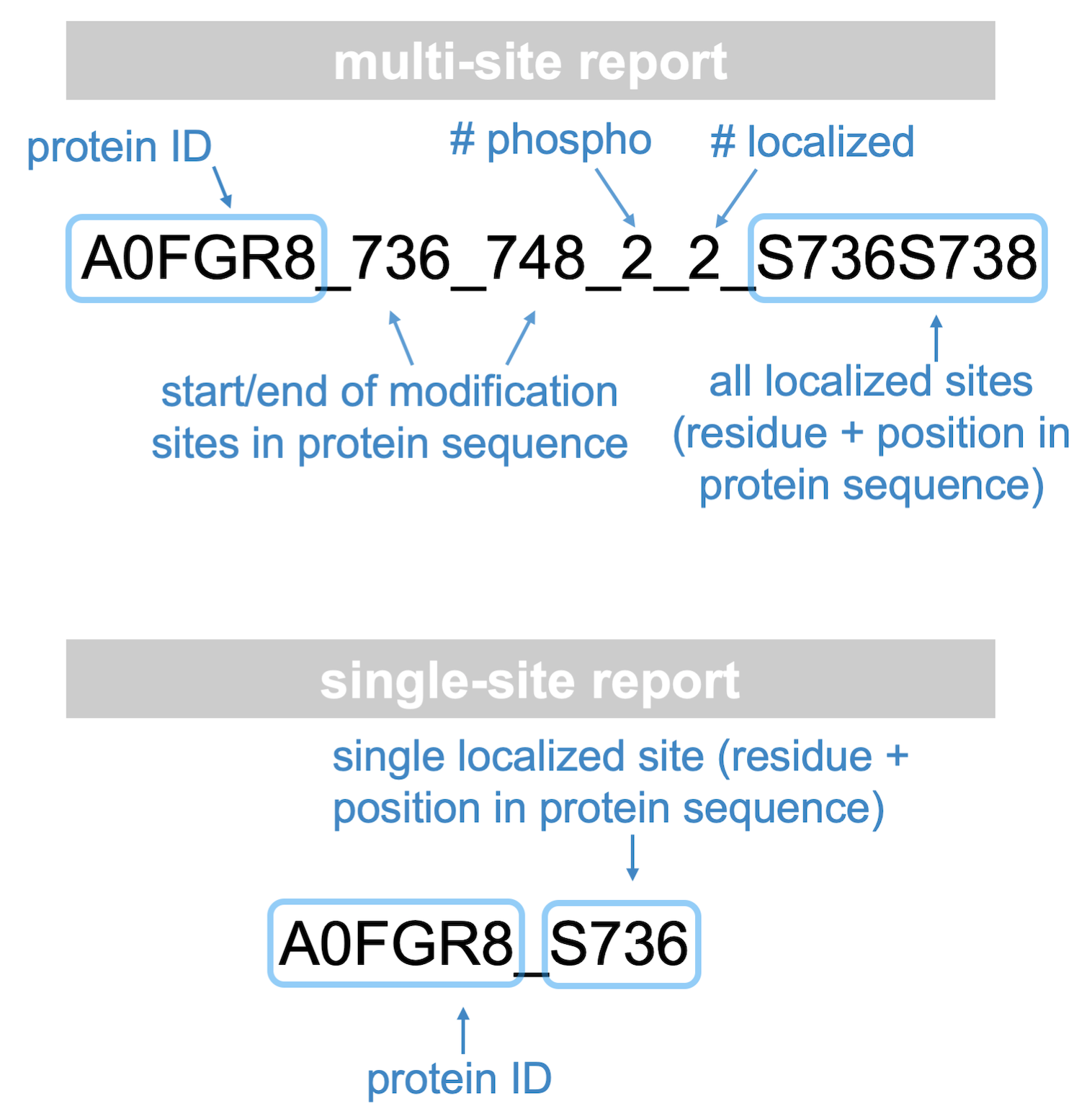
A key to the row indices in the resulting multi- and single-site reports is shown below.
Analyze the whole proteome samples
While you’re inspecting the results of the phosphorylation-enriched samples, you can set up the analysis of the unenriched (‘proteome’) samples. We will again use just two fractions each from two different TMT 10-plexes.
The files are organized similarly to the phospho data, so we can use the ‘Add folder recursively’ button again to load the data.
We can then use the ‘By parent directory’ button to get experiment labels like we did before. Instead of using the ‘TMT10-phospho-bridge’ workflow, select and load the ‘TMT10-bridge’ workflow.
On the ‘Quant (Isobaric)’ tab, the annotation files should load automatically.
Lastly, on the ‘Run’ tab, set the output location to be a new folder (‘my-tmt-proteome-results’) and click ‘RUN’.