Using FragPipe
FragPipe can be downloaded here. Follow the instructions on that same Releases page to launch the program.
Complete workflows are available for a variety of experiment types, we recommend starting your analysis with a built-in workflow, which can then be customized and saved for future use.
For partial processing (e.g. to save time upon re-analysis), steps can be skipped by unchecking the corresponding boxes. This tutorial walks through each tab in some detail, but once FragPipe is configured, analysis can be as simple as choosing spectral files, a database, and a workflow to run. Find a guide to output files here.
Before you get started, make sure your LC-MS file format is compatible with the workflows you want to perform. For Thermo data (with or without FAIMS), we recommend converting .raw files to mzML with peak picking. DIA data acquired with overlapping/staggered windows must be converted to mzML with demultiplexing.
Linux users: please note that Mono must be installed to directly read Thermo .raw files.
Bruker .d indicates ddaPASEF or diaPASEF files from timsTOF, other Bruker .d files should be converted to .mzML. Please also note that timsTOF data requires Visual C++ Redistributable for Visual Studio 2017 in Windows. If you see an error saying cannot find Bruker native library, please try to install the Visual C++ redistibutable.
| Workflow Step | .mzML | Thermo (.raw) | Bruker (.d) | .mgf |
|---|---|---|---|---|
| DIA-Umpire signal extraction | ✔ | ✔ | ||
| diaTracer signal extraction | ✔ | |||
| MSFragger search | ✔ | ✔ | ✔ | ✔ |
| MSFragger-DIA | ✔ | ✔ | ||
| Label-free quantification | ✔ | ✔ | ✔ | |
| SILAC/dimethyl quantification | ✔ | ✔ | ✔ | |
| TMT/iTRAQ quantification | ✔ | ✔ | ||
| Crystal-C artifact removal | ✔ | ✔ | ||
| PTMProphet localization | ✔ | ✔ | ✔ | |
| PTM-Shepherd summarization | ✔ | ✔ | ✔ | |
| Spectral library generation | ✔ | ✔ | ✔ | ✔ |
| DIA-NN quantification | ✔ | ✔* | ✔ |
FragPipe runs on Windows and Linux operating systems. While very simple analyses may only require 8 GB RAM, large-scale/complex analyses or timsTOF data will likely need 24 GB memory or more. Free disk space is needed to run FragPipe analyses and save reports, typically +20-50% of spectral file size for non-ion mobility data. Disk space requirements for quantification of timsTOF data are greater, +60% spectral file size if .d files are uncompressed, but up to +250% if Bruker’s compression function has been used.
Tutorial contents
- Configure FragPipe
- Select workflow and add spectral files
- DIA-Umpire SE
- Choose a sequence database
- Configure MSFragger search
- Validation
- PTMs
- Label-free quantification
- Isobaric quantification
- Spectral library generation
- DIA quantification with DIA-NN
- Run FragPipe
Configure FragPipe
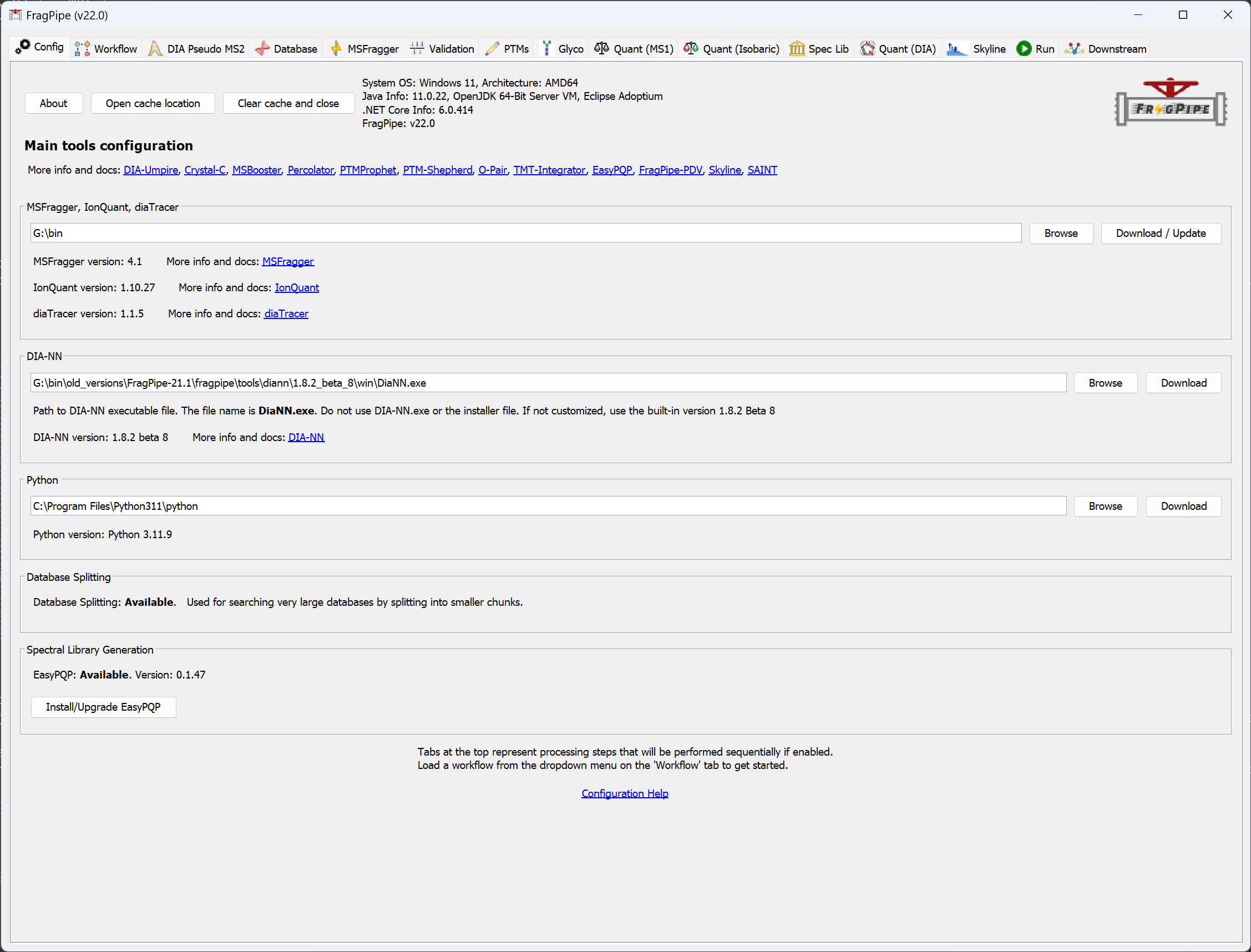
When FragPipe launches, the first tab in the window (‘Config’) will be used to configure the program.
- Connect FragPipe to a MSFragger.jar, IonQuant.jar, and diaTracer.jar program files. If you already have the latest versions and they are in the same folder, use the ‘Browse’ button to select the folder. Use ‘Download/Update’ to fetch the latest versions if you don’t have them.
- Optional: download and install the latest DIA-NN if you want. After installation, specify the path to
DiaNN.exein FragPipe. FragPipe bundles DIA-NN that should be good for most analysis. - Optional: Python is needed to perform database splitting (necessary in complex searches/low memory situations) and spectral library generation. If you already have Python 3.8 - 3.11 plus a few additional packages installed use ‘Browse’ to locate your python.exe file. ‘Download’ will take you to install Python. See Python installation help for details.
Note: FragPipe requires Python 3.8 - 3.11.
Select workflow and add spectral files
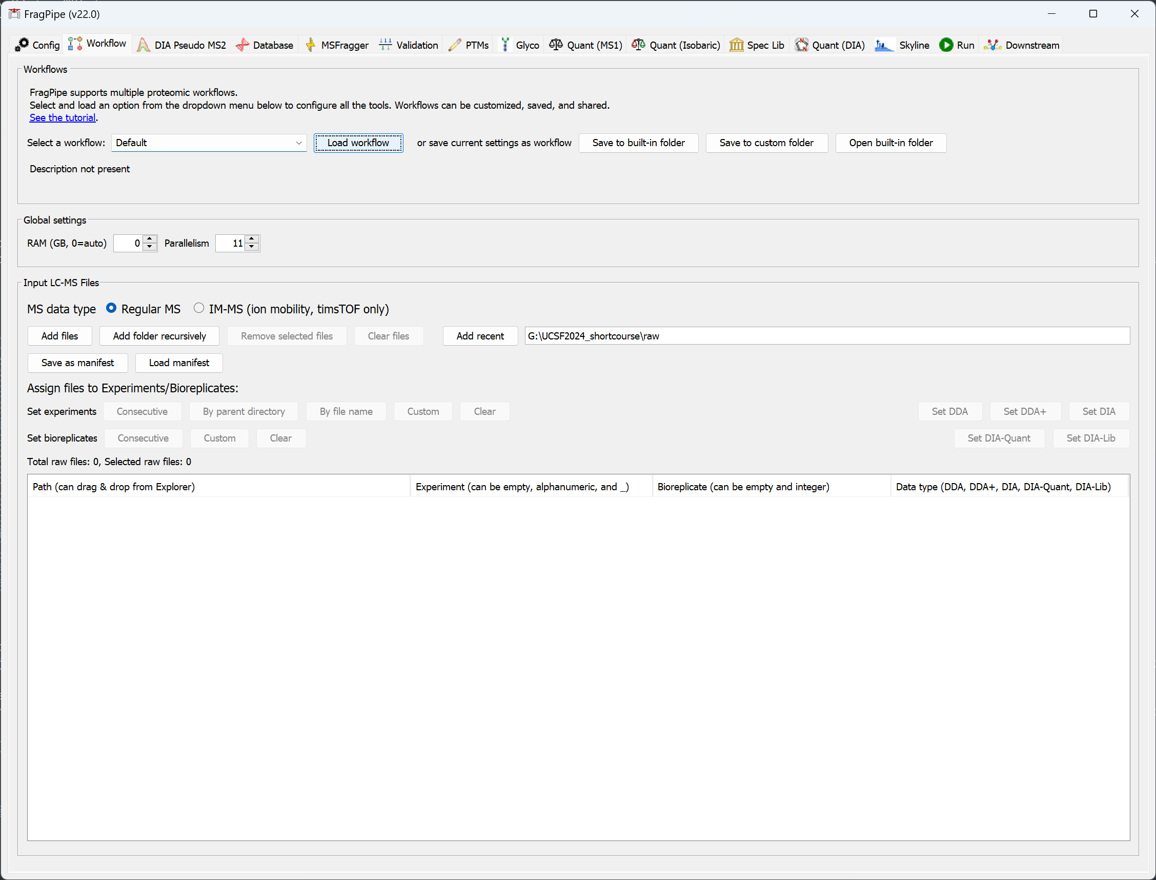
In the ‘Workflow’ tab:
-
Choose the workflow you want to use from the dropdown menu and press ‘Load’. Use the Default workflow for simple conventional (closed) searches. A number of common workflows (including glyco and DIA) are provided. We always recommend starting with one of the provided workflows and customizing it as needed. Customized workflows can be saved (with a unique name) for future use or sharing with other users (all workflows are stored in the FragPipe ‘workflows’ folder).
-
Set the amount of memory & number of logical cores to use. A RAM setting of 0 will allow FragPipe to automatically detect available memory and allocate a safe amount. Notes about HPC: On some high performance computing configurations, RAM=0 may be interpreted literally, so users should manually specify an appropriate amount of memory.
-
Select ‘IM-MS’ for Bruker timsTOF PASEF data or ‘Regular MS’ for all other data types (including FAIMS). Drag & drop LC/MS files into the window or use ‘Add files’ or ‘Add Folder Recursively’ to add all files in a folder, including those in subfolders.
Notes about timsTOF data: We recommend using raw ddaPASEF files (.d files), where the .d folder is the raw file. If you have already run MSFragger on the .d files, having the .mzBIN files from that analysis in the same directory as the .d files will speed up the analysis. If you don’t need to perform quantification, you can use .mgf files (which can be generated by Bruker’s instrument software immediately after data acquisition is completed) instead of .d.
Once you’ve loaded your spectral files, set the data type (DDA, DDA+, DIA, DIA-Quant, or DIA-Lib; hover over ‘Data type’ in FragPipe to view the tooltip with more information) and annotate your data to specify Experiment and Bioreplicates, which determines how your PSM/peptide/protein etc. reports will be generated (the ‘Save as manifest’ button stores file locations and annotations for future use):
Single-experiment report
Leave the ‘Experiment’ and ‘Bioreplicate’ fields blank. Use this option if you want to analyze all input files together and generate a single merged report (e.g., building a combined spectral library from all input data).
Multi-experiment report
Indicate the ‘Experiment’ and ‘Bioreplicate’ for each input file as shown below, where each replicate of two experimental conditions is composed of two fractions. Different fractions from the same sample should have the same ‘Experiment’/’Bioreplicate’ name.
| Path | Experiment | Bioreplicate |
|---|---|---|
| run_name_1.mzML | Control | 1 |
| run_name_2.mzML | Control | 1 |
| run_name_3.mzML | Control | 2 |
| run_name_4.mzML | Control | 2 |
| run_name_5.mzML | Treatment | 3 |
| run_name_6.mzML | Treatment | 3 |
| run_name_7.mzML | Treatment | 4 |
| run_name_8.mzML | Treatment | 4 |
Note: If you would like to use MSStats for downstream statistical analysis of FragPipe-generated reports, the ‘Bioreplicate’ ID (e.g., 1, 2, 3, and 4 in the table above) should not be reused by different replicates from different experiments. However, if each pair of ‘Control’ and ‘Treatment’ is from the same study subject (detailed discussion here), you should use the same ‘Bioreplicate’ ID for the corresponding ‘Control’ runs and ‘Treatment’ runs like this:
| Path | Experiment | Bioreplicate |
|---|---|---|
| run_name_1.mzML | Control | 1 |
| run_name_2.mzML | Control | 1 |
| run_name_3.mzML | Control | 2 |
| run_name_4.mzML | Control | 2 |
| run_name_5.mzML | Treatment | 1 |
| run_name_6.mzML | Treatment | 1 |
| run_name_7.mzML | Treatment | 2 |
| run_name_8.mzML | Treatment | 2 |
where ‘run_name_1.mzML’, ‘run_name_2.mzML’, ‘run_name_5.mzML’, and ‘run_name_6.mzML’ are controls and treatments from the same study subject; ‘run_name_3.mzML’, ‘run_name_4.mzML’, ‘run_name_7.mzML’, and ‘run_name_8.mzML’ are controls and treatments from another study subject.
Affinity-purification data
When analyzing AP-MS and related data (e.g. BioID) for compatibility with the Resource for Evaluation of Protein Interaction Networks (REPRINT), ‘Experiment’ names should be written as follows:
Negative controls: Put CONTROL in the Experiment column, and label each biological replicate with a different replicate number.
Bait IPs: Use [GENE]_[condition] format to describe the experiments, where [GENE] is the official gene symbol of the bait protein, e.g. HDAC5. If there are multiple conditions for the same bait protein (e.g. mutant and wt), add can add ‘condition’, e.g. HDAC5_mut.
| Path | Experiment | Bioreplicate |
|---|---|---|
| run_name_1.mzML | CONTROL | 1 |
| run_name_2.mzML | CONTROL | 2 |
| run_name_3.mzML | CONTROL | 3 |
| run_name_4.mzML | HDAC5 | 1 |
| run_name_5.mzML | HDAC5 | 2 |
| run_name_6.mzML | HDAC5 | 3 |
| run_name_7.mzML | HDAC5_mut | 1 |
| run_name_8.mzML | HDAC5_mut | 2 |
| run_name_9.mzML | HDAC5_mut | 3 |
Note: All negative controls should be labeled the same, as CONTROL, even if you have negative controls generated under different conditions or in different cell lines.
TMT/iTRAQ data
For TMT/iTRAQ analysis, spectral files should be in mzML format (with peak picking, see the conversion tutorial). Raw files are not currently supported.
TMT/iTRAQ experiments typically consist of one or more “plexes” (multiplexed samples), each composed of multiple spectral files (if samples were prefractionated). Use ‘Experiment’ to denote spectral files/fractions from the same plex while leaving the ‘Bioreplicate’ column empty. Different plexes must be organized into separate, uniquely-named folders. E.g., if you have 2 TMT plexes, with 2 spectral files (peptide fractions) in each, you can create a folder (e.g. named ‘MyData’), containing two subfolders (e.g. ‘TMT1’ and ‘TMT2’) each containing the corresponding mzML files. We recommend you load data by clicking ‘Add folder recursively’ and selecting ‘MyData’ folder, then assign files to Experiments/Groups ‘By parent directory’, resulting in the following spectral file annotation:
| Path | Experiment | Bioreplicate |
|---|---|---|
| run_name_tmt1_1.mzML | TMT1 | |
| run_name_tmt1_2.mzML | TMT1 | |
| run_name_tmt2_1.mzML | TMT2 | |
| run_name_tmt2_2.mzML | TMT2 |
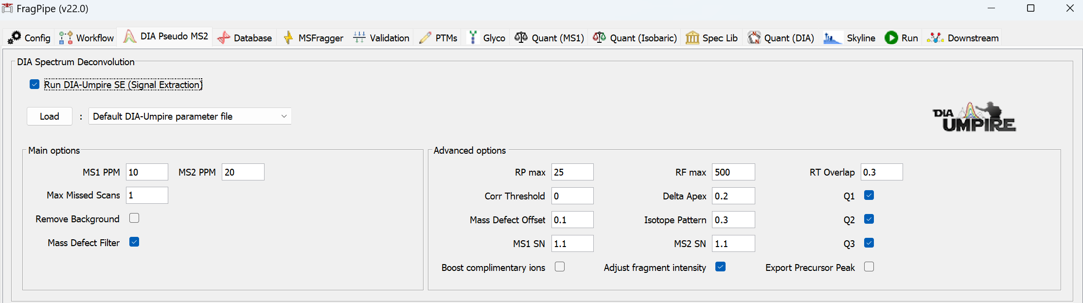
Run DIA-Umpire SE
DIA-Umpire’s signal extraction module can be used for .raw and .mzML files without ion mobility. See this tutorial for more detail.
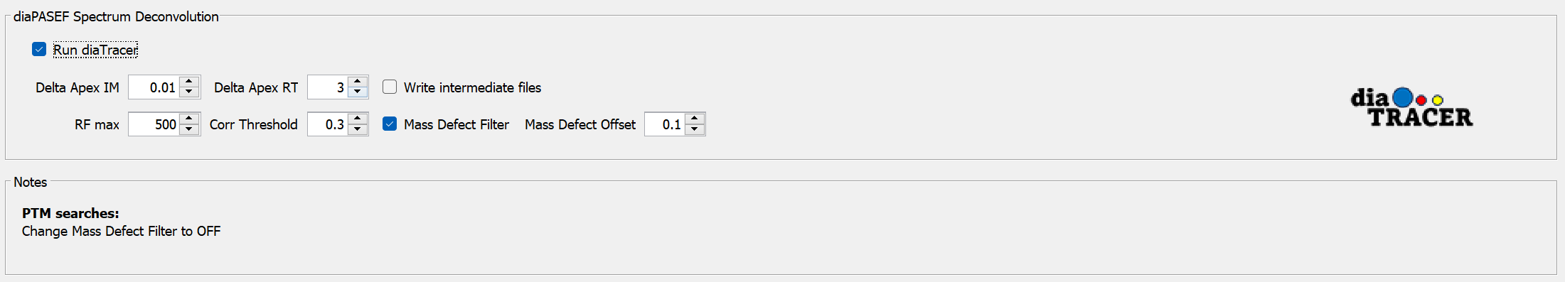
Run diaTracer
diaTracer’s signal extraction module can be used for diaPASEF .d files.
Specify a protein sequence database
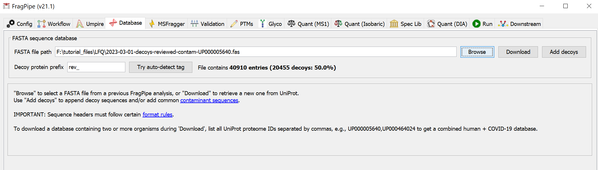
Use ‘Browse’ to select a FASTA file from a previous FragPipe/Philosopher analysis. If you haven’t made a database file using FragPipe/Philosopher before, select ‘Download’ to fetch one from UniProt. Choose database options and select an organism (use the UniProt proteome ID to specify your own, like ‘UP000000625’ for E. coli, or a comma-separated list of IDs, like ‘UP000005640,UP000464024’ for human+SARS-CoV-2). We generally recommend using ‘Reviewed’ sequences. Additional spike-in sequences from an existing FASTA file may be added. iRT sequences can be added as well (e.g., if you are building a spectral library for DIA analysis and added iRT peptides to your samples). Specify the download location, then choose ‘Select directory’ to download the database.
If you need to use a custom FASTA database, use the ‘Add decoys’ button to add decoys (common contaminants can also be added). FragPipe should show that 50% of the entries contain the decoy tag. Please note that sequence entry headers need to follow specific formatting, UniProt is generally recommended.
To combine two existing databases (e.g., custom protein sequence files A.fas and B.fas), follow the steps below:
1) Locate the Philosopher executable file (path can be found on the ‘Config’ tab).
2) Open a command line window and navigate to the folder with the two database files to be merged.
3) In this folder, run philosopher.exe workspace --init, where philosopher is the full path to the Philosopher executable file from step 1.
4) Next run philosopher.exe database --custom A.fas --add B.fas --contam.
Note that A.fas and B.fas should not contain decoys or contaminants. The --custom tag will automatically add decoy (reversed) sequences, and the --contam tag adds common contaminants.
5) Optionally, run philosopher.exe workspace --clean to delete intermediate files generated in these steps.
Configure MSFragger search
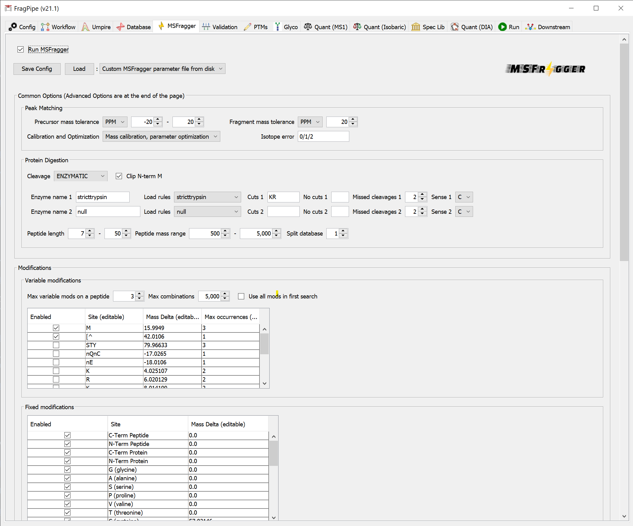
In the ‘MSFragger’ tab, you can check that the search parameters are suitable for your analysis. You can choose to save a customized parameter file to load for future use, or save the entire workflow (from the ‘Workflow’ tab).
Note about calibration and optimization: ‘Calibration and Optimization’ is set, by default, to “Mass Calibration, Parameter Optimization”. It will effectively perform multiple simplified MSFragger searches with different parameters to find the optimal settings for your data. In practice, it results in 5-10% improvement in the number of identified PSMs at the expense of increased analysis time. To save time, consider changing this option to “Mass Calibration” or even “None”, especially if you already know your data (e.g. from previous searches of the same or similar files) and can adjust the corresponding MSFragger parameters (fragment tolerance, number of peaks used, intensity transformation) manually, if needed.
Note about highly complex searches: For non-specific searches or for searches with many variable modifications, you may need to use the database splitting option, for which Python must be installed (see Configure FragPipe above).
Note about custom enzymes: To use an enzyme not listed in the digestion rules drop-down menu, use nonspecific from the ‘Load rules’ drop-down menu, enter the custom cleavage rules, then select ENZYMATIC from the ‘Cleavage’ drop-down menu.
Validation
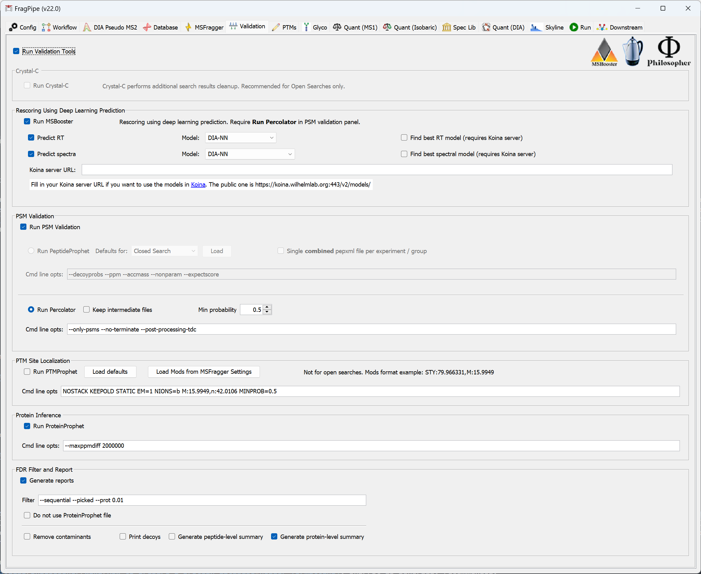
If you loaded one of the common workflow file provided with FragPipe, or previously updated the downstream parameters when setting MSFragger search parameters, you can skip to the next section. You can also load default downstream processing parameters by selecting the appropriate ‘Load defaults’ button. In most cases, search results from MSFragger must be filtered by PeptideProphet or Percolator and ProteinProphet. Percolator should perform better than PeptideProphet for low mass accuracy (e.g. ion trap) MS/MS data, and it is now the default option for all TMT workflows. Please note that Percolator is not compatible with open or mass offset searches, and may fail for extremely sparse datasets with few high-scoring PSMs.
For open search workflows, select Crystal-C to remove open search artifacts and improve the interpretability of your results (Note: at present, Crystal-C does not support .d files, and will be disabled by FragPipe when using .d as input).
MSBooster (new since v17.0) uses deep learning to predict additional features (including MS/MS spectra, retention time, detectability, and ion mobility) that can be used by Percolator to increase identifications, particularly from DIA and HLA data.
PTM-Prophet can be used to provide localization probabilities from closed search results. Load a TMT-phospho workflow to see the defaults or specify custom --mods using the format residues1:modmass1,residues2:modmass2 to provide the amino acids and their respective variable modifications. Mod masses should match those provided to the MSFragger search.
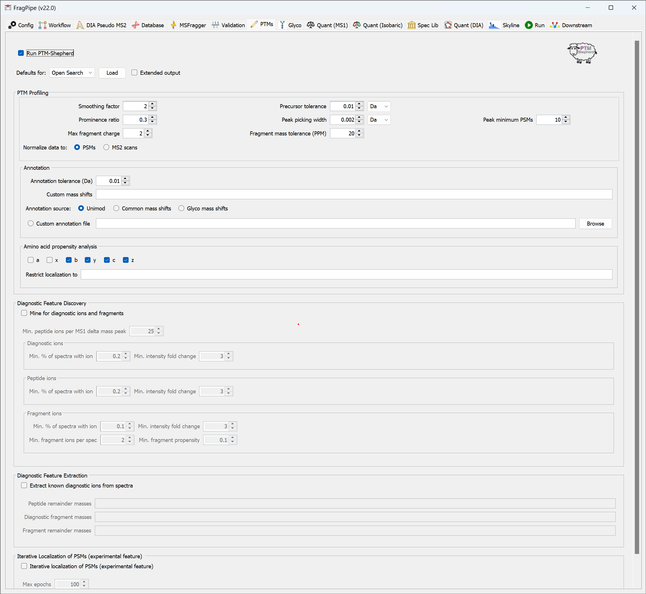
PTMs
For open search workflows, PTM-Shepherd summarizes delta masses and provides reports on residue localization, retention time similarity, and more. For glyco workflows, PTM-Shepherd provides multi-attribute glycan assignment and FDR control, see this section of the glyco tutorial for more detail.
LFQ: Label-free Quantification
To perform label-free quantification or stable isotope-based quantification (e.g., SILAC, dimethyl), make sure ‘Run MS1 quant’ is selected. Analyses performed without any quantification method selected will report spectral counts by default.
IonQuant is the default LFQ tool in FragPipe. Min ions (default = 1) controls how many quantifiable ions are required for protein-level quantification. Select a Protein quant option (either top-N, e.g. summation of the top 3 most intense peptides, or MaxLFQ approach. The latter is recommended). Match-between-runs (MBR) is available for closed search workflows.
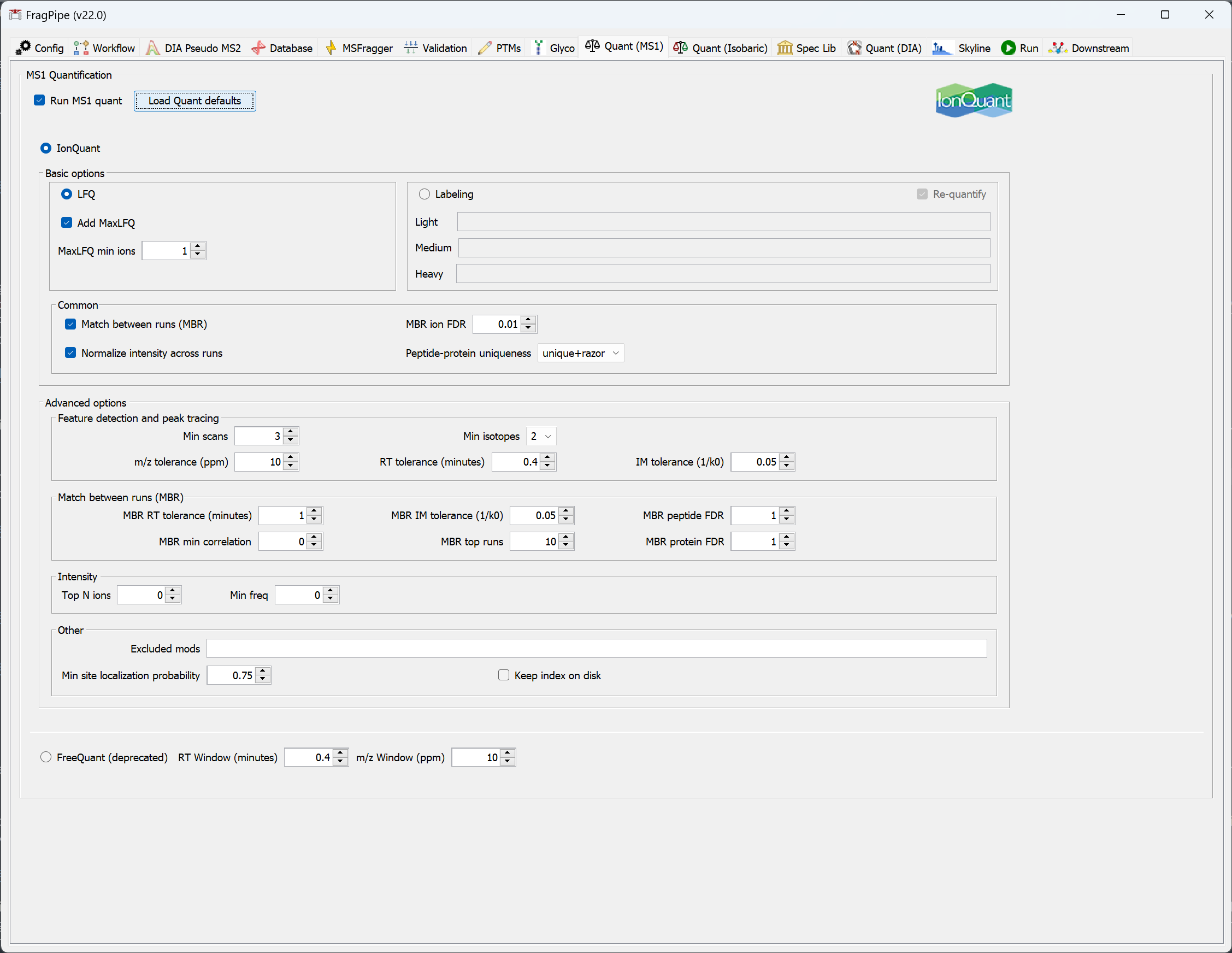
Note: IonQuant provides a lot of flexibility with how identifications are transfered between runs with MBR. Two of the key parameters controlling MBR are ‘MBR min correlation’ and ‘MBR top runs’. The MBR min correlation parameter allows matching only between runs with an overlap-weighted correlation (Spearman correlation of [retention time, intensity, and ion mobility] * overlap in IDs) above the specified threshold (0 by default). In addition, MBR top runs is applied to allow transfer of ions only from the highest N (by default 10) correlated runs that are above the ‘MBR min correlation’.
The optimal choice of MBR parameters depends on the experimental design. For example, in an AP-MS experiment with three replicates of Bait protein and 3 replicates of Negative Controls, one may want to set ‘MBR top runs’ parameter to 2, so only runs of the same kind can be used as donor runs for MBR. As a result, MBR will be performed only between Bait IP runs, or between the Control runs, but not between the two groups.
If you want to allow transfer between all runs in the dataset, set ‘MBR top runs’ to a large value (larger than the number of runs in the dataset) and set ‘MBR min correlation’ to 0.
MBR is FDR-controlled, we recommend 0.01 (i.e., 1%) ion-level FDR (default value). However, to allow more transfers (at the risk of introducing more quantification error/noise), MBR ion FDR can be relaxed, e.g. to 0.05 (5%).
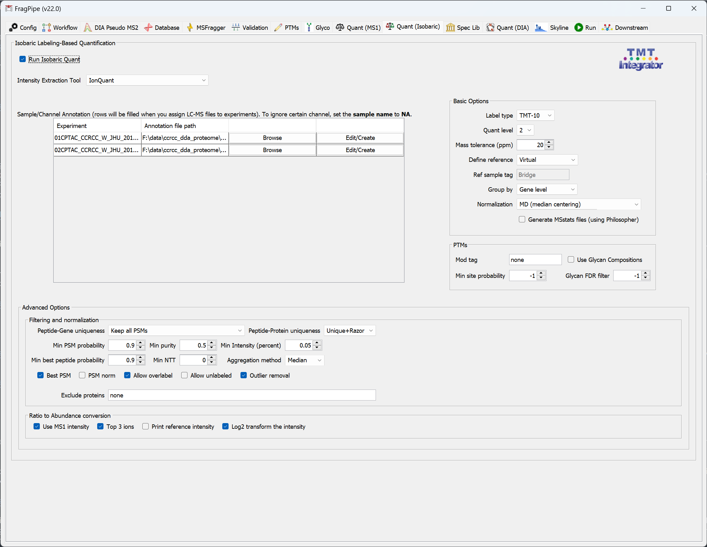
Isobaric Labeling-Based Quantification
To perform isobaric labeling-based quantification (TMT/iTRAQ),
- Check that the correct ‘Label type’ is selected (e.g. TMT10, TMT6, iTRAQ4, etc). If you need to change it at this point, we recommend going to the ‘Workflow’ tab and loading the correct workflow since the label also needs to be specified properly in the MSFragger search.
- For each experiment set in the ‘Workflow’ tab, select ‘Edit/Create’ Sample/Channel Annotation to assign sample information to each TMT/iTRAQ channel, or ‘Browse’ to load an existing ‘*annotation.txt’ file. (Each folder can have only one ‘*annotation.txt’ file, so be sure that fractions/replicates of each plex are in their own uniquely-named folder that corresponds to the experiment name. FragPipe will automatically find the right annotation file if these are set correctly.)
In the annotation pop-up window:
- Load the selected TMT/iTRAQ channels.
- Provide the experiment/replicate information for each channel.
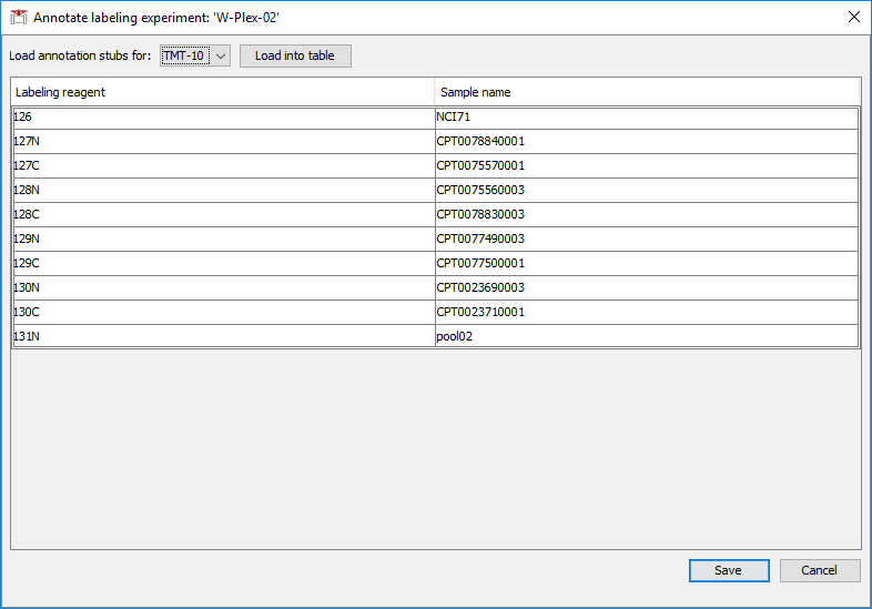
Annotation files will be named ‘annotation.txt’ and saved in each folder. Only one ‘annotation.txt’ is allowed per folder, so we recommend separate folders for each plex (see TMT/iTRAQ data above).
Note: Instead of naming samples/channels in FragPipe using Edit/Create, you can make annotation files in advance (as long as the file names end in ‘annotation.txt’), and FragPipe will load it automatically if it is in the same folder as the corresponding mzML files. When creating these files, make sure the value in first column (channel) and in the second column (sample) are separated with a space, not tab or any other character.
Note: If you have multiples plexes and added a common reference sample to each plex for bridging purposes, label these common reference samples as commonprefix_plexnumber (e.g. pool1, pool2, etc). If you want to use this common reference as the basis for computing the TMT/iTRAQ ratios for each PSM (within TMT-Integrator), select Reference sample from ‘Define reference’, and enter the text keyword describing the common reference channel (e.g. ‘pool’) that matches your naming scheme. Alternatively, select Virtual Reference if you do not have a reference sample. With the virtual reference approach, individual channel intensities for each PSM will be converted to ratios by dividing each channel intensity by the average intensity across all channels in that PSM.
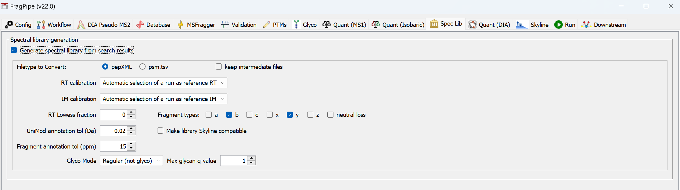
Spectral library generation
Spectral libraries can be generated within closed search-based workflows. A library will be generated for each experiment specified in the ‘Workflow’ tab. Experiments must contain more than one spectral file.
- Automatic selection of a run as reference RT selects the run with the most identified peptides as a reference. Overlapped peptides are used for the alignment
- Biognosys_iRT, ciRT, and Pierce_iRT uses the peptides from the Biognosys iRT kit, common human peptides, and Pierce iRT kit to perform the alignment
- For unfractionated data, Automatic selection of a run as reference RT is recommended
- When building the library from fractionated data, there may be not enough overlapped peptides for the alignment. Should consider using the other options.
- ciRT is overall the safest option for human samples
- Users can also provide their own iRT peptides by using the User provided RT calibration file option
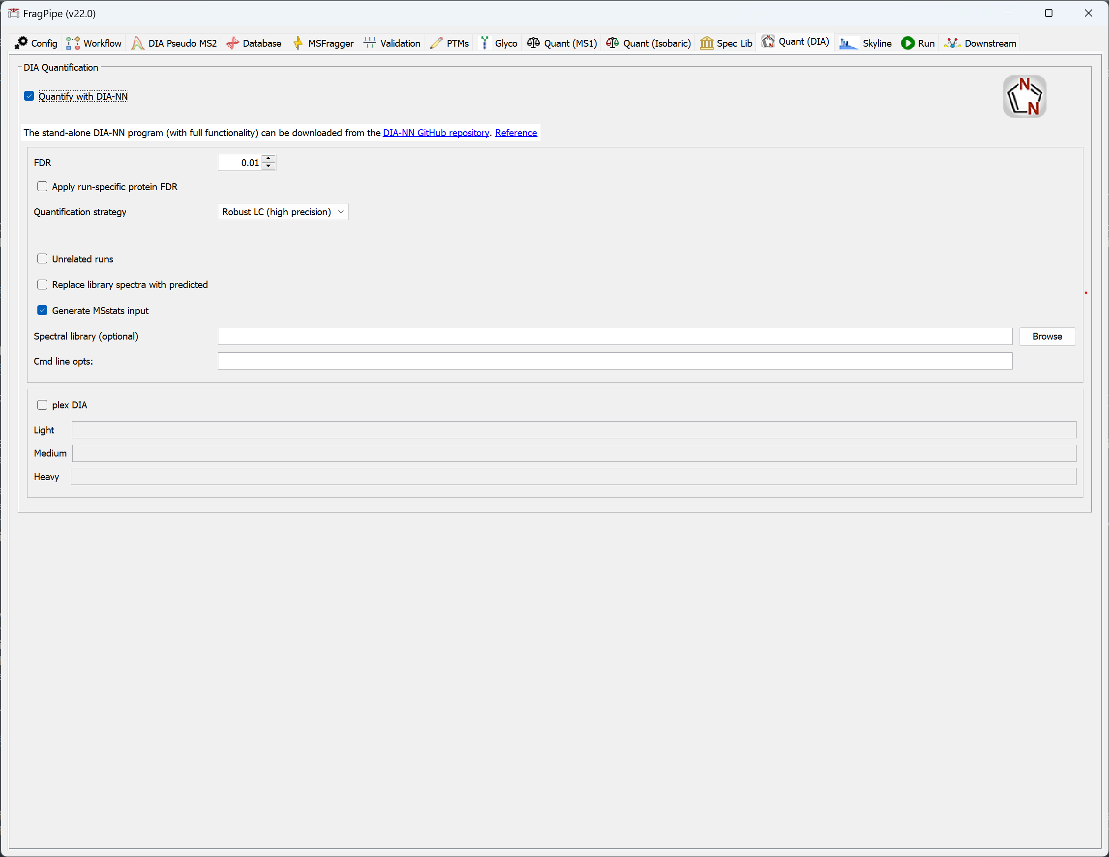
DIA quantification
DIA experiments can be quantified in FragPipe with DIA-NN. DIA files labeled with the ‘DIA-Quant’ data type on the Workflow tab will only be used for quantification (i.e. not used for spectral library building), files labeled ‘DIA’ or ‘GPF-DIA’ will be used for spectral library building and quantification if both steps are included in the workflow. See the DIA-NN documentation for more information on the ‘Quantification strategy’ options.
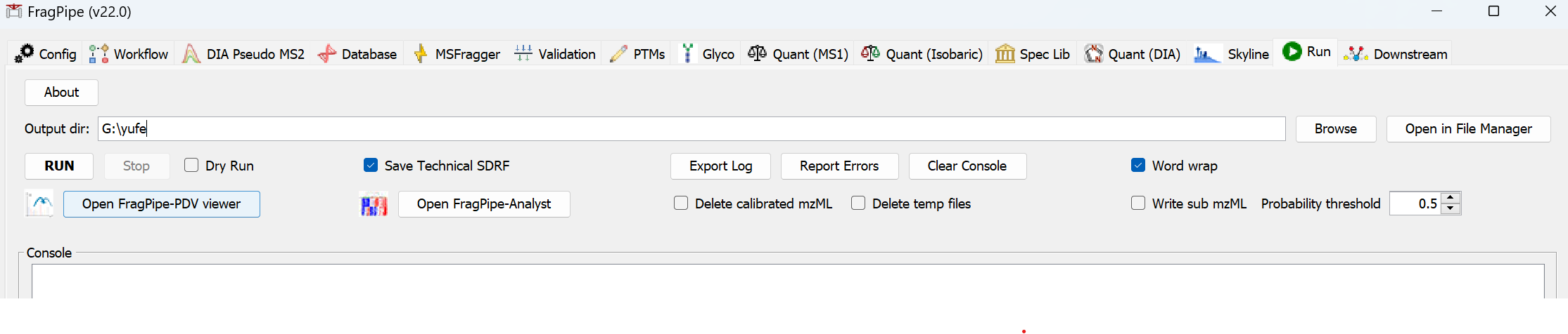
Run FragPipe
- Browse for the folder where you would like the search results to be written.
- Press ‘RUN’ to begin the analysis! A guide to output files can be found here. For more help, see the MSFragger wiki, FAQ, or search issues on Github.